
Blog
Numerical Computing Past Paper 2019 – BS 5th Term UOS (CS-3941)
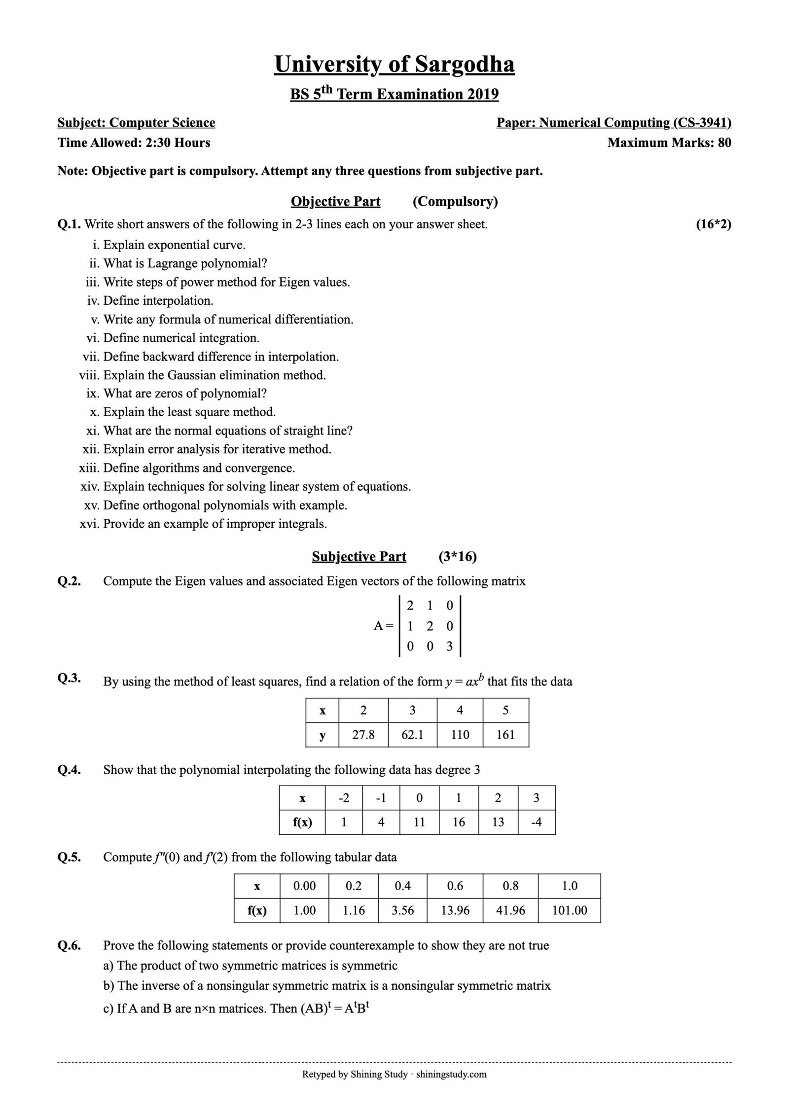
University of Sargodha (UOS) BS 5th term Numerical Computing (CS-3941) past paper 2019, with the full question paper in text form and step-by-step solved answers. All numerical results are checked with code.
Print / download (A4, high quality): Full-size paper
Numerical Computing Past Paper 2019 (text version)
University of Sargodha – BS 5th Term Examination 2019, Subject: Computer Science
Paper: Numerical Computing (CS-3941) · Time: 2:30 Hours · Maximum marks: 80
Note: Objective part is compulsory. Attempt any three questions from subjective part.
Objective part – Q1: Write short answers of the following in 2-3 lines each on your answer sheet. (16*2)
- Explain exponential curve.
- What is Lagrange polynomial?
- Write steps of power method for Eigen values.
- Define interpolation.
- Write any formula of numerical differentiation.
- Define numerical integration.
- Define backward difference in interpolation.
- Explain the Gaussian elimination method.
- What are zeros of polynomial?
- Explain the least square method.
- What are the normal equations of straight line?
- Explain error analysis for iterative method.
- Define algorithms and convergence.
- Explain techniques for solving linear system of equations.
- Define orthogonal polynomials with example.
- Provide an example of improper integrals.
Subjective part (3*16)
Q2. Compute the Eigen values and associated Eigen vectors of the following matrix
| 2 | 1 | 0 |
| 1 | 2 | 0 |
| 0 | 0 | 3 |
Q3. By using the method of least squares, find a relation of the form y = axb that fits the data
| x | 2 | 3 | 4 | 5 |
|---|---|---|---|---|
| y | 27.8 | 62.1 | 110 | 161 |
Q4. Show that the polynomial interpolating the following data has degree 3
| x | -2 | -1 | 0 | 1 | 2 | 3 |
|---|---|---|---|---|---|---|
| f(x) | 1 | 4 | 11 | 16 | 13 | -4 |
Q5. Compute f″(0) and f′(2) from the following tabular data
| x | 0.00 | 0.2 | 0.4 | 0.6 | 0.8 | 1.0 |
|---|---|---|---|---|---|---|
| f(x) | 1.00 | 1.16 | 3.56 | 13.96 | 41.96 | 101.00 |
Q6. Prove the following statements or provide counterexample to show they are not true
a) The product of two symmetric matrices is symmetric
b) The inverse of a nonsingular symmetric matrix is a nonsingular symmetric matrix
c) If A and B are n×n matrices. Then (AB)t = AtBt
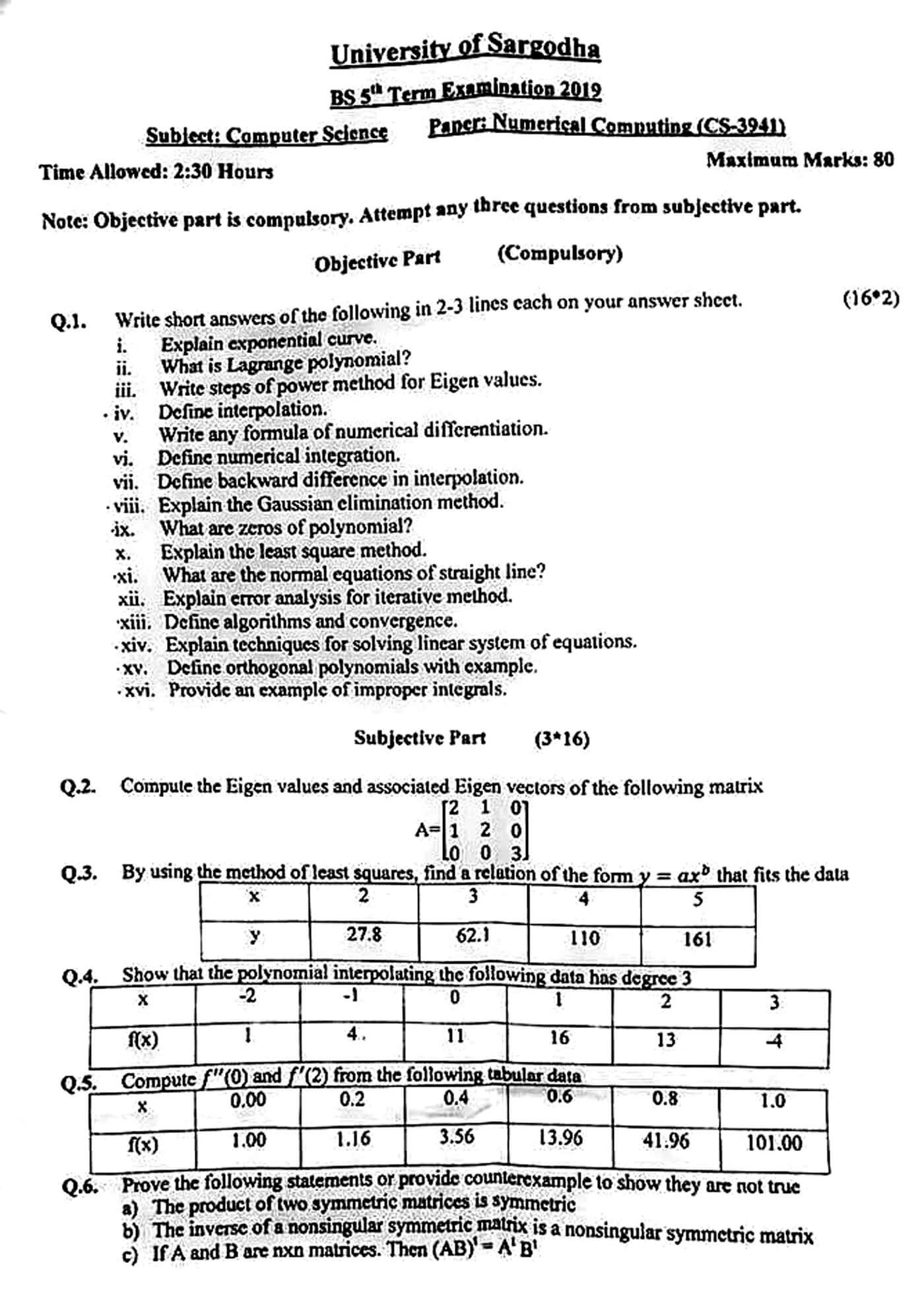
Original paper (scanned copy)
The clean paper above is retyped by Shining Study from this original University of Sargodha question paper. Click the scan to view it full size.
Solved answers
Q1 – Short questions
(i) Exponential curve: a curve of the form y = aebx (or y = abx), where the rate of change is proportional to the value itself – growth if b > 0, decay if b < 0. Taking logs gives a straight line (ln y = ln a + bx), which is how it is fitted by least squares.
(ii) Lagrange polynomial: the interpolating polynomial through n + 1 points written as P(x) = Σ f(xi) Li(x), where Li(x) = Πj≠i (x − xj)/(xi − xj). It works for unequally spaced points and has degree ≤ n.
(iii) Power method steps: (1) choose a starting vector x0 (e.g. [1,1,…,1]ᵀ); (2) compute y = A xk; (3) take λ = largest (absolute) component of y; (4) normalize xk+1 = y/λ; (5) repeat until λ and x stop changing. λ converges to the dominant eigenvalue and x to its eigenvector.
(iv) Interpolation: estimating the value of a function at a point between given tabulated points, by passing a polynomial (or other function) through the known data. Estimating outside the range is extrapolation.
(v) Numerical differentiation formula: central difference f′(x) ≈ [f(x + h) − f(x − h)]/(2h); also f″(x) ≈ [f(x + h) − 2f(x) + f(x − h)]/h². From Newton’s forward formula: f′(x0) ≈ (1/h)[Δy0 − Δ²y0/2 + Δ³y0/3 − …].
(vi) Numerical integration: approximating a definite integral ∫ab f(x)dx from function values at a set of points, when the antiderivative is hard or the function is only tabulated. Examples: trapezoidal rule, Simpson’s 1/3 and 3/8 rules, Gaussian quadrature.
(vii) Backward difference: ∇f(xi) = f(xi) − f(xi−1); higher orders ∇kf = ∇k−1f(xi) − ∇k−1f(xi−1). They are used in Newton’s backward interpolation formula for points near the end of the table.
(viii) Gaussian elimination: a direct method for Ax = b. Using row operations, the augmented matrix [A | b] is reduced to upper-triangular form (forward elimination, with pivoting for stability), then the unknowns are found by back substitution starting from the last equation. Cost ≈ n³/3 operations.
(ix) Zeros of a polynomial: the values of x for which P(x) = 0 (its roots). A polynomial of degree n has exactly n zeros, counting multiplicity and complex roots. Example: x² − 5x + 6 has zeros 2 and 3.
(x) Least squares method: finds the curve that best fits data by minimizing the sum of squares of the errors, S = Σ[yi − f(xi)]². Setting the partial derivatives of S to zero gives the normal equations, which are solved for the curve’s parameters.
(xi) Normal equations of a straight line y = a + bx: Σy = na + bΣx and Σxy = aΣx + bΣx².
(xii) Error analysis for iterative methods: the error at step k is ek = xk − x*. We check convergence by |xk+1 − xk| < tolerance or relative error |xk+1 − xk|/|xk+1|. The order of convergence p satisfies |ek+1| ≈ C|ek|p (bisection linear, Newton quadratic). Round-off and truncation errors are also considered.
(xiii) Algorithm and convergence: an algorithm is a finite, well-defined sequence of steps that solves a problem. An iterative algorithm converges if its sequence of approximations xk approaches the true solution as k → ∞; the rate at which it does so is the rate (order) of convergence.
(xiv) Techniques for linear systems: direct methods – Cramer’s rule, Gaussian elimination, Gauss–Jordan, LU decomposition (Doolittle, Crout, Cholesky); iterative methods – Jacobi, Gauss–Seidel, SOR, useful for large sparse systems.
(xv) Orthogonal polynomials: a set of polynomials {Pn} with ∫ab w(x)Pm(x)Pn(x)dx = 0 for m ≠ n. Example: Legendre polynomials on [−1, 1] with w = 1: P0 = 1, P1 = x, P2 = (3x² − 1)/2; ∫−11 x·1 dx = 0. Chebyshev polynomials are another example.
(xvi) Improper integral example: ∫1∞ 1/x² dx = 1 (infinite limit), or ∫01 1/√x dx = 2 (integrand unbounded at x = 0).
Q2 – Eigenvalues and eigenvectors
Characteristic equation: |A − λI| = 0
| 2-λ   1    0  |
|  1   2-λ   0  |  = (3-λ)[(2-λ)^2 - 1] = (3-λ)(λ-1)(λ-3) = 0
|  0    0   3-λ |
Eigenvalues: λ = 1, 3, 3.
λ = 1: (A − I)x = 0 gives x₁ + x₂ = 0 and 2x₃ = 0, so x = k(1, −1, 0)ᵀ.
λ = 3: (A − 3I)x = 0 gives −x₁ + x₂ = 0, x₁ − x₂ = 0, and x₃ is free. So x₁ = x₂ and x₃ is any value: x = k₁(1, 1, 0)ᵀ + k₂(0, 0, 1)ᵀ. Two independent eigenvectors: (1, 1, 0)ᵀ and (0, 0, 1)ᵀ.
Check: A(1,1,0)ᵀ = (3,3,0)ᵀ = 3(1,1,0)ᵀ ✓; A(1,−1,0)ᵀ = (1,−1,0)ᵀ ✓.
Q3 – Least squares fit y = axb
Take log₁₀: log y = log a + b log x, i.e. Y = A + bX with X = log x, Y = log y, A = log a.
| x | y | X = log x | Y = log y | X² | XY |
|---|---|---|---|---|---|
| 2 | 27.8 | 0.3010 | 1.4440 | 0.0906 | 0.4347 |
| 3 | 62.1 | 0.4771 | 1.7931 | 0.2276 | 0.8555 |
| 4 | 110 | 0.6021 | 2.0414 | 0.3625 | 1.2291 |
| 5 | 161 | 0.6990 | 2.2068 | 0.4886 | 1.5426 |
| Σ | 2.0792 | 7.4854 | 1.1693 | 4.0618 | |
Normal equations: 7.4854 = 4A + 2.0792b and 4.0618 = 2.0792A + 1.1693b.
Solving: b ≈ 1.930, A ≈ 0.8681, so a = 100.8681 ≈ 7.38.
Result: y ≈ 7.38 x1.93 (check: x = 4 gives 7.38 × 41.93 ≈ 108.8 ≈ 110 ✓).
Q4 – Degree of the interpolating polynomial
x     f(x)   Δf    Δ²f   Δ³f   Δ⁴f   Δ⁵f
-2     1
              3
-1     4           4
              7          -6
 0    11          -2            0
              5          -6           0
 1    16          -8            0
             -3          -6
 2    13         -14
            -17
 3    -4
The third differences are constant (−6) and the fourth and fifth differences are zero, so the interpolating polynomial has degree 3. (Indeed, it is P(x) = −x³ − x² + 7x + 11; e.g. P(2) = −8 − 4 + 14 + 11 = 13 ✓.)
Q5 – f″(0) and f′(2)
x     f(x)     Δ       Δ²      Δ³      Δ⁴     Δ⁵
0.0   1.00
              0.16
0.2   1.16            2.24
              2.40            5.76
0.4   3.56            8.00            3.84
             10.40            9.60            0
0.6  13.96           17.60            3.84
             28.00           13.44
0.8  41.96           31.04
             59.04
1.0 101.00
h = 0.2. Newton forward formula for the second derivative at x₀ = 0:
f″(0) = (1/h²)[Δ²y₀ − Δ³y₀ + (11/12)Δ⁴y₀] = (1/0.04)[2.24 − 5.76 + (11/12)(3.84)] = (1/0.04)(2.24 − 5.76 + 3.52) = 0.
The fourth differences are constant, so the data come from a 4th-degree polynomial. Newton’s forward polynomial with u = x/0.2 simplifies to f(x) = 1 + 100x⁴ (check: f(0.6) = 1 + 100 × 0.1296 = 13.96 ✓). Then f′(x) = 400x³, f″(x) = 1200x², so f″(0) = 0 ✓ and
f′(2) = 400 × 8 = 3200. (x = 2 is outside the table, so this uses the interpolating polynomial for extrapolation. If your paper meant f′(0.2), it is 400 × 0.008 = 3.2.)
Q6 – Prove or give a counterexample
(a) False. (AB)ᵀ = BᵀAᵀ = BA, which equals AB only if A and B commute. Counterexample: A = [[1,1],[1,0]], B = [[1,0],[0,0]] (both symmetric). AB = [[1,0],[1,0]], which is not symmetric.
(b) True. Let A be symmetric (Aᵀ = A) and nonsingular. A⁻¹ exists and is nonsingular since A⁻¹A = I (its inverse is A). Transposing AA⁻¹ = I gives (A⁻¹)ᵀAᵀ = I, i.e. (A⁻¹)ᵀA = I. So (A⁻¹)ᵀ is the inverse of A, and by uniqueness (A⁻¹)ᵀ = A⁻¹. Hence A⁻¹ is symmetric. ∎
(c) False. The correct rule is (AB)ᵀ = BᵀAᵀ. Counterexample: A = [[1,1],[0,0]], B = [[1,0],[1,0]]. AB = [[2,0],[0,0]], so (AB)ᵀ = [[2,0],[0,0]], but AᵀBᵀ = [[1,0],[1,0]]·[[1,1],[0,0]] = [[1,1],[1,1]] ≠ (AB)ᵀ.
Answers prepared by Shining Study for revision. Check them against your class notes and teacher’s guidance.